Appendix

A. Prefix trees

Our main result is achieved by reducing a tree inclusion problem to the following problem.

String prefix matching.  Consider the following computational problem over strings. Let $\Sigma$ be a finite alphabet and consider $\mathcal{W} = (\Sigma^*)^w$ the set of $w$-tuples of strings over $\Sigma$. For a string tuple $(s_1, \dots, s_w) \in \mathcal{W}$ and a set of string tuples $\mathcal{D} \subseteq \mathcal{W}$, the $w$-dimensional string prefix matching consists in finding the set

This string problem can be solved using a $w$-dimensional prefix tree. We give a short introduction to prefix trees for the string case but refer to standard literature for more details Knuth, 1999Donald Knuth. 1999. The Art of Computer Programming: Sorting and Searching, Volume 3. Addison-Wesley, Reading MA.

One-dimensional prefix tree.  Let $P_1, \dots, P_\ell \in \mathcal{A}^\ast$ be strings on some alphabet $\mathcal{A}$. Given an input string $s\in\mathcal{A}^\ast$, we wish to find the set of patterns $\{ P_{1 \leq i \leq \ell} | P_i \subseteq s\}$, i.e. $P_i$ is a prefix of $s$.

The prefix tree of $P_1, \dots, P_\ell$ is a tree with a tree node for each prefix of a pattern. The children of an internal node are the strings that extend the prefix by one character. The root of the tree is the empty string. Each tree node also stores a list of matching patterns, with each pattern stored in the unique corresponding node. Every prefix tree has an empty string node, which is the root of the tree. For every inserted pattern of length at most $L$ nodes are inserted, one for every non-empty prefix of the pattern. Thus a one-dimensional prefix tree has at most $\ell \cdot L + 1$ nodes and can be constructed in time $O(\ell \cdot L)$.

Given an input $s \in \mathcal{A}^\ast$, we can find the set of matching patterns by traversing the prefix tree of $P_1, \dots, P_\ell$ starting from the root. We report the list of matching patterns at the current node and move to the child node that is still a prefix of $s$, if it exists. This procedure continues until no more such child exists. In total the traversal takes time $O(|s|)$, as every character of $s$ is visited at most once.

Note that in theory the number of reported pattern matches can dominate the runtime of the algorithm. We can avoid this by returning the list of matches as an iterator, stored as a list of pointers to the tree nodes matching lists.

Multi-dimensional prefix tree.  A $w$-dimensional prefix tree for $w > 1$ is defined recursively as a one-dimensional prefix tree that at each node stores a $w-1$-dimensional prefix tree. Given an input $w$-tuple $(s_1, \dots, s_w) \in (\mathcal{A}^\ast)^w$, the traversal of the $w$-dimensional prefix tree is done by traversing the one-dimensional prefix tree on the input $s_1$ until no child is a prefix of the input, and then recursively traversing the $w-1$-dimensional prefix tree on $(s_2, \dots, s_w)$. Similarly to the one-dimensional case, the list of matching patterns is stored at prefix tree nodes and reported during traversal. The traversal thus takes time $O(|s_1| + \cdots + |s_w|)$, as every character of $s$ is visited at most once.

For $\ell$ tuples of size $w$ of words of maximum length $L$, we can bound the number of nodes of the $w$-dimensional prefix tree by $1 + (\ell \cdot L)^w$. The runtime and space complexity of the construction of the $w$-dimensional prefix tree is thus in $O((\ell \cdot L)^w)$, summarised in the result:

B. Lower bound on the number of patterns

In the regime of interest, $w$ is small, so the assumption $w \leq o(2^d)$ is not a restriction.

Proof

Let $w, d > 0$ and $\Delta \geq 4$ be integers. We wish to lower bound the number of port graphs of depth $d$, width $w$ and maximum degree $\Delta$. It is sufficient to consider a restricted subset of such port graphs, whose size can be easily lower bounded. We will count a subset of CX quantum circuits, i.e. circuits with only $CX$ gates, a two-qubit non-symmetric gate. Because we are using a single gate type, this is equivalent to counting a subset of port graphs with vertices of degree 4. Assume w.l.o.g that $w$ is a power of two. We consider CX circuits constructed from two circuits with $w$ qubits composed in sequence:

• Fixed tree circuit: A $\log_2(w)$-depth circuit that connects qubits pairwise in such a way that the resulting port graph is connected. We fix such a tree-like circuit and use the same circuit for all CX circuits. We can use this common structure to fix an ordering of the $w$ qubits, that refer to as qubits $1,\dots,w$.
• Bipartite circuit: A CX circuit of depth $D = d - \log_2(w)$ with exactly CX gates, each gate acting on a qubit and a qubit .

The following circuit illustrates the construction:

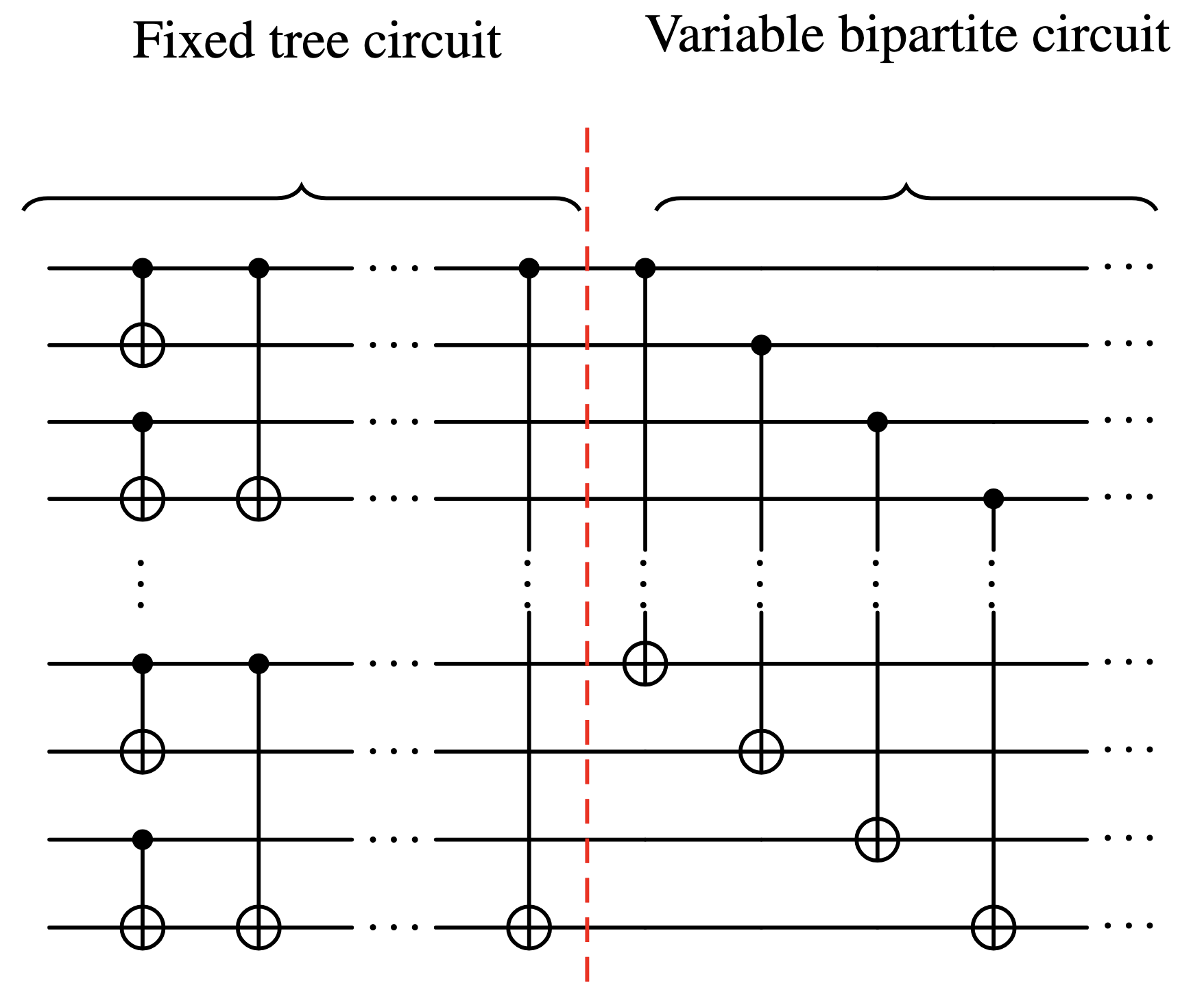
All that remains is to count the number of such bipartite circuits. Every slice of depth 1 must have $w / 2$ CX gates acting on distinct qubits. Every qubit $1$ to $w/2$ must interact with one of the qubits $w/2+1$ to $w$, so there are $(w/2)!$ such depth 1 slices. Repeating this depth 1 construction $D$ times and using Sterling’s approximation, we obtain a lower bound for the number of port graphs of depth $d$, width $w$ and maximum degree at least 4:

$$\left(\left(\frac{w}2\right)!\right)^D > \sqrt{w\pi}\left(\frac{w}{2e}\right)^{wD/2} = \left(\frac{w}{2e}\right)^{\Theta(w\cdot d)}$$

where we used $w = o(2^d)$ to obtain $\Theta(D) = \Theta(d)$ in the last step.